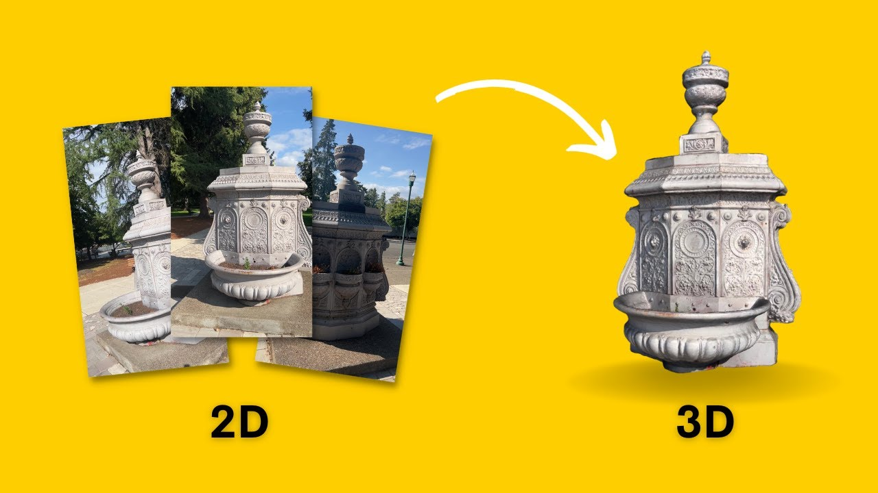
Imagine taking a few dozen photos of a room with your smartphone and, within minutes, having a complete 3D model you can walk through from any angle. That is 3D scene reconstruction — the science of transforming flat, 2D images into volumetric, navigable representations of real-world environments. This technology powers self-driving cars (mapping roads in real-time), augmented reality (placing virtual furniture in your living room), robotics (helping robots understand their surroundings), and special effects (recreating real sets in digital form).
But how does a machine, which sees only pixels, infer the three-dimensional structure of a scene? The answer lies in a combination of geometry, optics, and machine learning. This post explores the core techniques: Structure from Motion (SfM), Multi-View Stereo (MVS), depth sensing, neural radiance fields (NeRFs), and Gaussian splatting. We will examine how each method reconstructs depth, texture, and shape from images.
The Fundamental Challenge: Depth from Flat Images
A standard camera captures a 2D projection of a 3D world. When you take a photo, you lose the depth dimension entirely. A distant mountain and a nearby tree can occupy the same pixel coordinates. Reconstructing 3D requires solving the inverse problem: given multiple 2D projections from different viewpoints, recover the original 3D structure.
This is possible because of parallax — the apparent shift of objects against a background when the observer moves. Your brain uses parallax from your two eyes to perceive depth (stereopsis). Cameras do the same thing: compare images from slightly different positions to triangulate distances.
Scene Point P (x, y, z)
        /\
       /  \
      /    \
     /      \
    /        \
Camera Left   Camera Right
  (Image L)     (Image R)
If you know the geometric relationship between two cameras (their relative position and orientation), and you can identify the same 3D point in both images, you can triangulate its exact 3D coordinates using trigonometry.
Structure from Motion (SfM): The Backbone of 3D Reconstruction
Structure from Motion is the foundational technique for reconstructing 3D scenes from unordered image collections. SfM simultaneously solves for two unknowns: the 3D structure of the scene and the camera poses (position and orientation) for each image.
The SfM Pipeline
Step 1: Feature Detection and Description
The first step finds distinctive points in each image that can be reliably matched across views. The most common detector is SIFT (Scale-Invariant Feature Transform), which identifies corners, blobs, and edges that remain recognizable under rotation, scale changes, and lighting variations.
import cv2
import numpy as np

# Load two images of the same scene from different angles
img1 = cv2.imread('scene_view1.jpg')
img2 = cv2.imread('scene_view2.jpg')

# Initialize SIFT detector
sift = cv2.SIFT_create()

# Detect keypoints and compute descriptors
kp1, des1 = sift.detectAndCompute(img1, None)
kp2, des2 = sift.detectAndCompute(img2, None)

# Each keypoint has: (x, y) coordinates, scale, orientation
# Each descriptor is a 128-dimensional vector capturing local texture
Each image yields thousands of keypoints. A good keypoint is repeatable (found in multiple images) and distinctive (unlikely to be confused with another point).
Step 2: Feature Matching
The algorithm compares descriptors across image pairs using Euclidean distance. The best match for a point in image A is the point in image B with the most similar descriptor vector.
# FLANN matcher for efficient matching
FLANN_INDEX_KDTREE = 1
index_params = dict(algorithm=FLANN_INDEX_KDTREE, trees=5)
search_params = dict(checks=50)

flann = cv2.FlannBasedMatcher(index_params, search_params)
matches = flann.knnMatch(des1, des2, k=2)

# Apply Lowe's ratio test to filter ambiguous matches
good_matches = []
for m, n in matches:
    if m.distance < 0.75 * n.distance:
        good_matches.append(m)
A match suggests that two pixels in different images correspond to the same physical point in the scene.
Step 3: Estimating the Fundamental Matrix and Camera Pose
Given a set of matched points, the algorithm estimates the essential matrix (for calibrated cameras) or fundamental matrix (for uncalibrated cameras). This 3x3 matrix encodes the geometric relationship between two camera views.
From the essential matrix, the algorithm decomposes it into rotation (R) and translation (t) — the relative pose between cameras. This step uses the 8-point algorithm or 5-point algorithm (more robust).
# Estimate essential matrix from matched points
essential_matrix, mask = cv2.findEssentialMat(
    pts1, pts2, camera_matrix,
    method=cv2.RANSAC, prob=0.999, threshold=1.0
)

# Recover camera pose (rotation and translation)
_, rotation, translation, _ = cv2.recoverPose(
    essential_matrix, pts1, pts2, camera_matrix
)
Step 4: Triangulation
With two camera poses known, each matched point pair yields a 3D point by intersecting rays. The solution finds the point that minimizes reprojection error — the distance between the observed pixel and the projection of the 3D point into each image.
def triangulate_point(P1, P2, pt1, pt2):
    """
    P1, P2: 3x4 camera projection matrices
    pt1, pt2: 2D points in homogeneous coordinates
    """
    # Build matrix A for linear triangulation
    A = np.array([
        pt1[0] * P1[2] - P1[0],
        pt1[1] * P1[2] - P1[1],
        pt2[0] * P2[2] - P2[0],
        pt2[1] * P2[2] - P2[1]
    ])

    # Solve using SVD
    _, _, V = np.linalg.svd(A)
    point_3d = V[-1] / V[-1, 3]  # Homogeneous to Cartesian
    return point_3d[:3]
Step 5: Bundle Adjustment
After initial reconstruction, bundle adjustment globally optimizes all camera poses and 3D points simultaneously. It minimizes the sum of squared reprojection errors across all images using non-linear least squares (Levenberg-Marquardt algorithm).
Error = Σ Σ ||observed_pixel_ij - project(camera_i, point_j)||²
         i j

Where:
- i iterates over cameras
- j iterates over 3D points visible in camera i
- project() projects a 3D point into image coordinates
Bundle adjustment is computationally expensive but essential for accurate reconstructions. Tools like Ceres Solver (Google) and g2o (OpenSLAM) provide optimized implementations.
Multi-View Stereo (MVS): Dense Reconstruction
SfM produces a sparse point cloud — typically thousands of points. Multi-View Stereo densifies this into millions of points by computing depth for every pixel in every image.
MVS assumes camera poses are already known (from SfM). For each pixel in a reference image, MVS searches along the epipolar line in neighboring images to find the depth that maximizes photometric consistency (pixels look the same across views).
# Simplified depth map computation
def compute_depth_pixel(ref_img, neighbor_img, ref_cam, neighbor_cam, x, y):
    best_depth = None
    best_score = float('inf')

    # Search over depth hypotheses
    for depth in np.arange(0.5, 100.0, 0.1):
        # Project pixel into 3D at candidate depth
        point_3d = ref_cam.unproject(x, y, depth)

        # Project 3D point into neighbor image
        x2, y2 = neighbor_cam.project(point_3d)

        # Compare pixel neighborhoods using NCC (Normalized Cross-Correlation)
        ref_patch = extract_patch(ref_img, x, y, patch_size=7)
        neighbor_patch = extract_patch(neighbor_img, x2, y2, patch_size=7)

        score = 1 - normalized_cross_correlation(ref_patch, neighbor_patch)

        if score < best_score:
            best_score = score
            best_depth = depth

    return best_depth
PatchMatch Stereo is the state-of-the-art MVS algorithm. It uses random initialization followed by spatial propagation — good depth estimates spread to neighboring pixels like a virus, converging in 3-5 iterations.
Active Depth Sensing: Structured Light and LiDAR
Passive methods rely on natural texture. Textureless white walls, glass, or shiny surfaces break them. Active sensors project their own light patterns to measure depth directly.
Structured Light (Microsoft Kinect v1, Intel RealSense) projects infrared dot patterns onto the scene. A camera observes how the pattern distorts. By comparing to a known reference pattern, depth is computed via triangulation. This works well indoors but fails in sunlight.
LiDAR (Light Detection and Ranging) sends laser pulses and measures return time. For each point, depth = (speed of light × time of flight) / 2. LiDAR generates dense, accurate point clouds even in complete darkness. Modern iPhone Pro models include LiDAR for AR. Autonomous vehicles use 64-128 beam rotating LiDARs for 360-degree perception.
# LiDAR principle simplified
def calculate_distance(time_of_flight_ns):
    speed_of_light = 299_792_458  # m/s
    distance = (speed_of_light * (time_of_flight_ns * 1e-9)) / 2
    return distance  # meters
Neural Radiance Fields (NeRF): The AI Revolution
In 2020, researchers at UC Berkeley introduced NeRF — a neural network that learns a continuous volumetric representation of a scene from sparse images. NeRF produces photorealistic novel views with correct lighting, reflections, and transparency.
NeRF represents a scene as a function F: (x, y, z, θ, φ) → (RGB, σ)
- Input: 3D position (x,y,z) + viewing direction (θ,φ)
- Output: Color (RGB) and volume density (σ)
The network is a multilayer perceptron (MLP) with 8-10 layers. Training requires 50-200 images and 12-48 hours on a single GPU. Rendering a single novel view requires sampling hundreds of points along each camera ray and integrating the predicted colors.
# Simplified NeRF ray marching
def render_nerf_ray(ray_origin, ray_direction, nerf_model):
    """Returns RGB color for a single camera ray"""
    colors = []
    densities = []

    # March along the ray from near to far
    for t in np.linspace(near, far, num_samples=128):
        point_3d = ray_origin + ray_direction * t

        # Query NeRF network
        rgb, density = nerf_model.predict(point_3d, ray_direction)
        colors.append(rgb)
        densities.append(density)

    # Volumetric rendering (alpha compositing)
    final_color = volume_rendering_integral(colors, densities)
    return final_color
NeRF Limitations: Extremely slow (seconds per frame), requires per-scene training (cannot generalize to new scenes without retraining), and assumes static scenes.
Instant-NGP (NVIDIA) reduced training to seconds using multi-resolution hash encoding. 3D Gaussian Splatting (2023) replaced NeRF's neural network with explicit Gaussian primitives, achieving real-time (100+ FPS) rendering with comparable quality.
Depth from Monocular Video: The Modern Approach
Recent advances use deep learning to estimate depth from single images or monocular video. This is an ill-posed problem (infinite 3D scenes map to the same 2D image), but neural networks learn priors from massive datasets.
MiDaS (Mixed Depth and Scale) is a popular monocular depth estimation model:
import torch
model = torch.hub.load('intel-isl/MiDaS', 'MiDaS_small')

def estimate_depth(rgb_image):
    # Normalize and resize to model input (384x384 or 512x512)
    input_tensor = preprocess(rgb_image)

    with torch.no_grad():
        depth_map = model(input_tensor)

    # depth_map contains relative depth (near = high value, far = low value)
    return depth_map
Monocular depth produces relative depth (pixel A is twice as far as pixel B) but not absolute metric depth. Combining monocular depth with SLAM (Simultaneous Localization and Mapping) yields metric reconstruction.
Applications of 3D Scene Reconstruction
Autonomous Vehicles use real-time reconstruction to understand road geometry, detect obstacles, and localize within HD maps. LiDAR and cameras work together — LiDAR provides accurate depth, cameras provide texture for semantic segmentation (pedestrian vs. traffic sign).
Augmented Reality (AR) requires understanding the environment to place virtual objects realistically. ARKit (Apple) and ARCore (Google) reconstruct planes, estimate lighting, and track surfaces in real-time on smartphones.
Cultural Heritage Preservation scans historical sites and artifacts. The Notre Dame Cathedral was extensively scanned with LiDAR years before the 2019 fire, enabling precise digital reconstruction for restoration.
Robotics uses 3D reconstruction for navigation, manipulation, and exploration. A robot vacuum builds a map of your home. A warehouse robot tracks pallets in 3D space. A Mars rover reconstructs terrain to avoid hazards.
Film and Visual Effects create digital doubles of actors and real sets. The "bullet time" effect in The Matrix involved 120 cameras arranged in a circle, reconstructing the scene from every angle simultaneously.
Practical Reconstruction Pipeline with COLMAP
COLMAP is the most widely used open-source SfM and MVS software. A typical pipeline:
# 1. Extract SIFT features from all images
colmap feature_extractor --database_path database.db --image_path images/

# 2. Match features between image pairs
colmap exhaustive_matcher --database_path database.db

# 3. Run incremental SfM reconstruction
colmap mapper --database_path database.db --image_path images/ --output_path sparse/

# 4. (Optional) Dense reconstruction with MVS
colmap image_undistorter --image_path images/ --input_path sparse/0/ --output_path dense/
colmap patch_match_stereo --workspace_path dense/ --workspace_format COLMAP
colmap stereo_fusion --workspace_path dense/ --workspace_format COLMAP --output_path dense/fused.ply
The output fused.ply is a dense 3D point cloud viewable in software like MeshLab, Blender, or CloudCompare.
Accuracy Metrics and Challenges
Reconstruction accuracy is measured by:
- Completeness – Percentage of the scene captured
- Precision – Geometric error vs. ground truth
- Recall – How many true surfaces were reconstructed
Current state-of-the-art (COLMAP + PatchMatch) achieves sub-millimeter precision for small objects and centimeter precision for building-scale scenes.
Key challenges remain:
- Specular surfaces (glass, mirrors) – Light reflects away from the camera
- Textureless regions (white walls, snow) – No features to match
- Dynamic scenes – Moving people or cars violate the static-scene assumption
- Large-scale reconstruction – Processing thousands of images requires hours or days
Final Thoughts
3D scene reconstruction has progressed from laboratory curiosity to everyday technology. Your smartphone performs real-time reconstruction for AR filters. Autonomous vehicles navigate using LiDAR and camera fusion. Drones map construction sites in minutes. Cultural heritage sites are digitally preserved for future generations.
The trend is clear: real-time, accurate, and generalizable reconstruction is becoming ubiquitous. NeRF and Gaussian Splatting are pushing toward photorealistic rendering from casual captures. Monocular depth estimation is improving rapidly, potentially eliminating the need for multiple cameras.
Understanding these techniques — SfM, MVS, active sensing, neural fields — is essential for anyone working in computer vision, robotics, AR/VR, or autonomous systems. The ability to transform pixels into 3D geometry is one of the most powerful capabilities in modern computing. As cameras become cheaper and compute becomes faster, the line between the physical world and its digital reconstruction will continue to blur.
The next time you see a self-driving car navigate a busy intersection or a phone measure the dimensions of a room, remember: behind that magic is geometry, optimization, and decades of research into how machines can learn to see the world in three dimensions.